Fig. 2. Compartmentalization model of Lake Ontario (adapted from Joe DePinto's Lake Ontario Model.

Back to Top

In early 2001, the Council approached the conveners of the Lake Erie Millennium Plan regarding the hosting of another modelling workshop that would complement themes of the concurrent Lake Erie in the Millennium- Progress and New Issues and Detroit River State of the Strait binational Conference planned for March of that year. Those conferences culminated in a roundtable discussion and workshop to address the question:

"What is the likely role of Detroit River remediation on the Lake Erie ecosystem?"

Accordingly, the Council hosted a second workshop immediately following the conclusion of that discussion to determine how a modelling approach would contribute answers to that question. Nine panelists with expertise in Great Lakes modelling were asked to attend the morning workshop and then make presentations during the modelling workshop. In addition to providing general comments on their opinion of the morning's proceedings, the panelists were asked to provide information regarding the following questions:

Back to Top

In early 2001, the Council approached the conveners of the Lake Erie Millennium Plan regarding the hosting of another modelling workshop that would complement themes of the concurrent Lake Erie in the Millennium- Progress and New Issues and Detroit River State of the Strait binational Conference planned for March of that year. The Lake Erie in the Millennium Conference brought together more than 130 people including researchers, government and agency representatives, and the public to discuss current research, progress, and new issues on Lake Erie. On the morning of March 29, a roundtable discussion and workshop on the "Influence of the Detroit River on the Lake Erie ecosystem" was completed at the Lake Erie in the Millennium - Progress and New Issues binational conference. Participants in breakout sessions identified key features and tests necessary to evaluate the question:

Telephone: 734-332-1200

email: jdepinto@limnotech.com

William G. Booty

NWRI, Environment Canada, 867 Lakeshore Rd.,

Burlington, ON L7R 4A6

Telephone: 905-336-4718

email: bill.booty@cciw.ca

Miriam Diamond

University of Toronto, Dept. of Geography,

100 St. George Street, Toronto, ON M5S 3G3

Telephone: 416-978-1586

email: diamond@geog.utoronto.ca

David M. Dolan

University of Wisconsin - Green Bay, 2420 Nicolet Drive,

Green Bay, WI 54311-7001

Telephone: 920-465-2986

email: doland@uwgb.edu

Kenneth G. Drouillard

University of Windsor, Great Lakes Institute for Environmental Research,

2990 Riverside Drive East, Windsor, ON N9B 3P4

Telephone: 519-253-3000 ext. 3446

email: kdrouillard@trent.ca

Russell G. Kreis Jr.

MED US - EPA, Large Lakes Research Station,

9311 Groh Road, Grosse Ile, MI 48138

Telephone: 734-692-7615

email: kreis.russell@epa.gov

Heather A. Morrison

Environment Canada, 4905 Dufferin St.,

Downsview, ON M3H 5T4

Telephone: 416-739-4761

email: heather.morrison@ec.gc.ca

Back to Top

Joseph V. DePinto, Limno-Tech, Inc.

Q1. The need for models.

Introduction to the Workshop:

This workshop follows up the previous IJC report, "Great Lakes Modeling Summit: Focus on Lake Erie " (CGLRM, 2000) of the summit held at IAGLR, 1999. Included in this document was a series of papers that described the feasibility of building an aquatic ecosystem model for Lake Erie that could examine the ecosystem-level effects of multiple stressors acting in concert. Today's workshop builds on the previous modelling summit while focussing more on the western basin of Lake Erie, and more specifically on the Detroit River/ Lake Erie system (CLGRM, 2000).

A number of important observations have been made at the Lake Erie in the Millennium conference (March 27-28, 2001). For example, the total phosphorus levels in the lake appear to be increasing. Is this observation the result of increased loadings or of changes in in-lake processing of phosphorus loads?

What I hope we can try to do in the future is to take observations like the phosphorus concentration trends and the statements and convert them into quantitative hypotheses that can be tested within a modelling framework. We can then make informed decisions on what needs to be done and what priorities need to be made in order to improve the system.

The charge for the afternoon is to ask:

What is the likely role of Detroit River remediation on the Lake Erie ecosystem?

This is a management question, although it is very generic in nature. To use a model to address this question we must get more specific. We must address questions like:

If we want to remediate the Detroit River so as to improve Lake Erie as well;

Where should we focus?

Where should we start?

Where should we spend our money?

How can specific potential remediation alternatives be simulated within a modelling framework?

But with regard to the Lake Erie Millennium Plan, models also have great value as research tools. Models are an integral part of the scientific method. Models serve as a means of quantitatively synthesizing process-related experimental results and theory along with field observations into a whole-system hypothesis-testing pool. With complex ecosystems, it becomes virtually impossible to measure ecosystem structure and functioning at the scale necessary to test hypotheses strictly with data; this is where system-level models have great value. While we can never really simulate the entire ecosystem, we can mathematically reproduce our conceptual model of the key processes and feedbacks as a means of testing system response to conditions that may exist but for which we do not have empirical experience. The great value of models used in this research mode is the knowledge gained when they "fail". In this way, gaps in our data or understanding are indicated. Then we can iterate between monitoring/experimentation and model application in order to build our understanding of how the ecosystem responds to external stimuli.

The challenge, of course, is how do we go about establishing a management model and a research model in a single framework. Often, the demands for spatial and temporal and kinetic (process) resolution in a research model may be very different than a management model. For example, a management model for PCBs might just look at total PCBs. However, this is generally not appropriate for a research study. For research purposes, we might want to look at the behaviour of some of the PCB congeners individually. These things make it a challenge to address both a management and a research model question in the same program.

With that bit of introduction, I will ask each of our panel members to address a specific modelling question related to our overall theme of modelling ecological change in the Detroit River - Lake Erie corridor.

In food web type models, we encompass large spatial scales. Hydraulic engineers use a different scale. In the case of the Detroit River, the engineers have divided the river into 20,000 cells. Ken considers it a single cell for modelling food web and contaminant dynamic processes. In terms of temporal scale, Ken uses a one-year time step whereas engineers use hours.

Do organisms respond to water quality changes in small time scales? How do we bring that into context?

Another aspect is the need for validation of our models to test the fit of the model to the monitoring data across spatial and temporal scale.

At some point we produce data to evaluate a model.

We need to continue monitoring programs to determine how well observations fit predictions. We monitor water and use mussels as biomonitors of bioavailable concentrations of contaminants. This permits us to integrate complex types of exchanges between water and sediment, which will let us determine time scale-specific absorption and desorption rates and flow rate changes. Flow changes over the course of hours, but desorption occurs over minutes.

There is also the matter of continuing monitoring so we have adequate data sets. We should couple the toxicokinetic models with hydrology models. One unifying approach is to use a single GIS framework to integrate the different types of models.

Questions:

Dave Culver: How did you link together these types of scales?

Answer: We used a compromise solution for the different biological compartments, and a hazard assessment approach. But we recognize that this is not a real picture of what is going on. It will continue to be a challenge coupling these models with biological profiling, i.e., linking modellers with biologists, and incorporating the physical and chemical aspects of the river environment.

Joe DePinto: We don't necessarily need to run hydrodynamic models together and then aggregate output to chemistry and biology.

Back to Top

The larger system is changing very rapidly and there are a number of important trends. We know that an increasing proportion of the population is urbanized. Emission rates are increasing. The amount of monitoring information data and infrastructure to monitor are both decreasing. An essential piece of the puzzle is missing--public buy-in. The public's concern and involvement is important and the government needs to maintain this. The university sector is not doing this. There is general loss of confidence in government ability to regulate new chemicals, new pharmaceuticals, and personal care products. We have fewer regulations and less compliance monitoring. In its place there are increasing numbers of voluntary actions that are not as effective as old policy.

We also need to look at expertise. In the government, we lost many people in 1994 when the two levels of government (Federal and Provincial) destroyed programs and information, data follow-up, and surveillance. We now have fewer really smart people going into environmental and engineering programs than ever before. This is an important piece of the puzzle in predicting where we are going to go.

Mass Balance Models link stressors (provide link) to effects and to impact.

Management generates policy, research does the science, and advocacy is the remaining group. The role of advocacy is in alerting the public that resource use is going to go beyond the carrying capacity.

We need to broaden the boundary of models to include the public, i.e. put people into the model. People are a stressor as well as being impacted on. We are moving from point source to nonpoint source emitters, with people increasingly becoming the problem.

Bob Costanza at Maryland has been working on watershed-to-watershed export to incorporate people. We need to clearly establish the chain of command in regards to motivating people to put effective policies into place.

We need to define research questions:

What is the effect of past actions? e.g. sediment dredging;

What is the effect of human population and resource use?

What is the effect of land use changes?

We lack the scientific basis to make a rationale for optimal land use. We need to reduce impacts

with patterns of living. We must evaluate past vs. the present with regard to future sources and trends. We need to learn from past problems such as phosphorus. For the phosphorus issue we had a problem, we found solutions, and we developed models to remedy problems. We need to integrate other issues such as lake hydrology, ice cover, and climate change.

Miriam's suggested approach is to run a series of coupled models such as watershed, river and lake, food web, human exposure, indicators, bioavailable metals as well as background versus anthropogenic loads to close the loop relating emissions and their effects.

We need to look at nutrients, persistent materials, and metals (speciation). What is the form of available compounds e.g. phosphorus? We need to add endocrine disruptors, pharmaceuticals, and personal care products to the list of chemicals that require modelling.

We need to do some screening to incorporate management questions into complex models to ensure that we address managers' research needs.

We can learn from past models such as the phosphorus model, so that we don't reinvent the wheel. A GIS model is a good approach.

Can one model address all issues? Yes, if we use coupled models.

One individual needs to grasp all components to be sure that individuals modelling each component don't go off on tangents and not connect. We need to retain some intellectual control and management over the overall enterprise. We also need to make continued use of, and improve, existing models.

Joe - idea of also advocacy models

The idea of open modelling, i.e., doing modelling in front of public, is important for communication and to keep us on track. We should be sharing data with the public. Also, model construction and application should be done this way and could potentially be used to promote scientific modelling.

The short answer is no, because as Russ Kreis mentioned there is a whole list of reasons why one monitors. Data that is collected for regulatory purposes is not often that useful for calibrating and confirming a quantitative and management level model. Although Joe is not sure what to do, his feeling is that we need to try to find a way to serve multiple masters. At the 1999 Modelling Summit the following recommendation was developed:

"Sufficient monitoring programs and coordinated research programs are essential to the development of modeling projects which can provide assistance to managers in addressing pressing management issues" (CGLRM, 2000).

If this means adapting or spending more money then we need to do that. Modellers need to be brought into the process earlier on so that they can be involved in planning data collection that will serve both management and model development needs.

Mass balance models can truly integrate the physics and biology of systems. And in order for mass balance to work, we need to measure more than concentration of the chemical of interest. We need to really understand where water is moving in the system. From Dave Culver and Bob Heath, we are asked to determine how bottom velocities and vertical mixing factor in to the effect of zebra mussels on nutrients, etc. There are important physical and biological interactions like this that up until recently we had not grasped. Questions like these that are being asked require more than the coarse-scale circulation patterns that we conventionally have used in our water quality modelling. We now need to implement fine-scale hydrodynamic models to give us the necessary information for our water quality models. Fortunately, advances in computer technology have made this hydrodynamic-water quality linkage feasible.

In its most fundamental form, a mass balance model is a computation of a concentration of the spatial and temporal profile of a substance. The very simplest form is a load ("W" ng/day) and a series of processes that operate on that load ("a"; an operator has units of a flow) in order to get a concentration, "C".

C[ng/m 3 ] = W[ng/day]/a[m 3 /day]

If we want to model to forecast a concentration we have to know the loads and the processes that are operators on the loads. We need to calibrate the model by making measurements in the system and then adjusting coefficients in the processes operator (a) that will "convert" our measured load into the observed concentrations. If we don't know the loads well, then the calibration process will be flawed. Message: We can't do forecasting or predictive mass balance models unless we measure the loads as accurately as possible.

Back to Top

Earlier, a point was made that we had to carry out solutions to management problems within a decision framework. We have done this for the last 15 years starting with acid rain, where everything is done within a Decision Support System called RAISON, (http://www.cciw.ca/nwri/software/raison.html) developed by our group at the Environment Canada's National Water Research Institute (NWRI).

The Great Lakes Toxic Chemical Decision Support System (GLTCDSS) is an example of an application which operates within RAISON. The system includes tools such as GIS, database, statistics, neural networks, expert systems, graphical displays, etc.

Using his laptop computer, Bill showed the interface of the GLTCDSS. This allows one to pick any of the Great Lakes or connecting channels, and automatically links the user to the appropriate database tables.

Miriam Diamond mentioned that there are different types of models needed for different systems/needs; a public user interface requires an order of magnitude more work to program than a technical user interface.

Most of work has been done on Lake Ontario; especially longterm monitoring by Joe DePinto and Bill Booty. The GLTCDSS contains a number of models;

* Don Mackay's and Miriam Diamond's regional fugacity model and * Rate Constant mass balance model * a regional air transport model * and 2 Lake Ontario models; LOTOX1 and LOTOX2.

The user can go through the system, extract the necessary information, and construct (in proper format) the data needed for the model.

All kinds of data (emissions, loadings, and ambient) are in the database already. We can extract data for whatever time period is necessary.

Here, one can choose one's lake and chemical, and then assign names to files that will be generated; for example, Lake Ontario PCBs. Here, we have all of the key parameters and values listed. We can change rate constants and have summary of all inputs. The same thing can be done for food chain; fish. As well, a mass balance diagram is generated.

Having all of the tools and interfaces set up in one system, makes it easy to quickly run different scenarios or do "gaming".

Bill Booty then showed some results that illustrated what Joe DePinto was talking about.

The RATECON model operates in a number of different modes. One can carry out steady state calculations of concentrations using loadings as inputs. It may also be run in reverse, using measured system concentrations to calculate what the loads should be.

For this example, measured system concentrations for the year 1995 are used as input to back-calculate the terrestrial loadings. It is assumed that the atmospheric loadings are known.

The model was initially calibrated starting with information known from the literature and the necessary loadings were determined. Many loadings were based initially from estimates taken from the literature. The model was then run backwards to see what loadings would be required to generate the measured outflow loads measured as part of the Niagara River Upstream/Downstream Program at Fort Erie.

The model was calibrated based on PCB loadings of 750 kg/y + 166 kg/y. from atmospheric sources. From this, Bill predicted 34 kg/y output from the lake, but the measured value is 219kg/y. The terrestrial load required to generate the 219 kg/y value is calculated to be 5700 kg/y. Where's the problem (750 vs 5700)? Is it the model? The data?

Similar discrepancies occur for other compounds as well. The estimated outflow for Hg is 325 kg/y. The observed amount is 550 kg [numbers are conservative], assuming highest credible resuspension levels. For Benzo [a] pyrene, the predicted level is 260 kg/y. The measured level is 150 kg/y.

Metals loadings should be an order of magnitude higher than reported to generate the output loads that have been measured at Fort Erie. Therefore, there must be problems either in loading estimates or in model parameterization. There are still lots of problems. If we don't know the loadings, we're in big trouble.

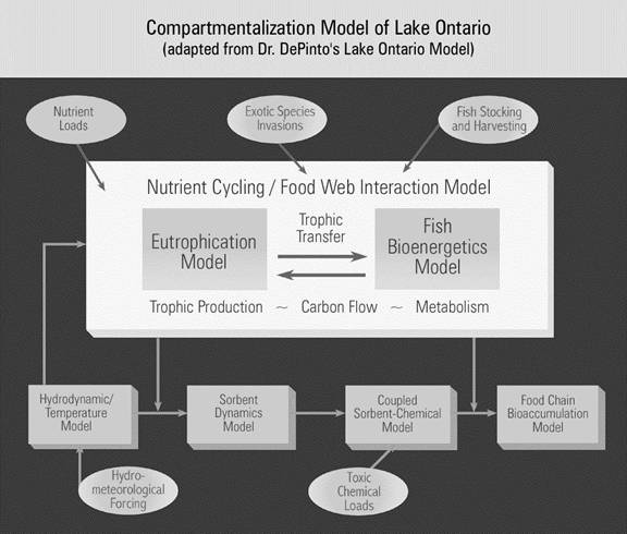
Response to Question : compartments

Bill showed an overhead (Fig. 2) ('adapted' from Joe DePinto's model of Lake Ontario compartmentalization model).

Missing compartments include fish, exotic species, hydrodynamic models, and temperature. We need hydrometerological forcing functions. Much of the function definition has been done. We need only to link the functions.

Joe DePinto: possibly two things are happening

1. When the measured outflow exceeds modelled outflow at steady state, the model could be wrong. For example, perhaps the system isn't at steady state. It may be responding to levels from 10 years ago. That doesn't help with Lake Ontario, which is a dynamic model.

2. The measurement data just aren't necessarily representative of what you think is being measured. Don't automatically blame the model.

It is also important to make sure you can't achieve a match. For example, by adding processes that you weren't aware of before. It may be a missing load rather than a transfer coefficient, or a short circuit in the lake. We are always faced with dilemmas if we don't have confidence in the model.

Back to Top

Russ believes that development of a decision support system is the way to go. We need a framework or a continuum that relates to everything people do, i.e., monitoring, assessment, experimentation, and the whole process of restoration. This system would aid management in making decisions about remediation.

Russ' perspective is from that of the EPA - an enforcement and regulatory agency. Credibility and reliability are paramount, because many of these issues end up in courts. It is different to go before a judge and enforce a $1B decision than to argue at a scientific meeting.

The whole Lake Erie initiative is part of this system and feeds into the bigger picture.

A modelling framework integrates physical, biological, chemical, and ecosystem dynamics.

Forecasting is paramount to any initiatives, even the work we've discussed today and in other work groups, too. The situation is "how do you know that event 'x' is going to happen if factor 'y' changes?" What will be the effects on Lake Erie? How do you know with any credibility?

We are often hoping against hope, and we use the lake scientific background to justify our hopes. Development will go ahead whether we like it or not. Forecasting and evaluation of various scenarios is absolutely critical (e.g., to estimate how many years it will be before can eat fish, given sediment concentration A vs. B).

This is part of the decreasing support system. All of these things flow together. They are a series of linked or coupled models that work together, as was the case for Lake Erie Models presented at the Case Western University workshop. They include submodels that help us understand things like surface waves, contamination, water quality, and food chain biomagnification.

Along with Joe DePinto, I believe that as the overhead was presented (Fig. 2), we have lots of information on contaminant models, but we should be dovetailing energetics models to serve two functions at once. For example, if Diporeia are gone, what are likely effects on lake trout? and what are implications for contaminant loads?

Russ agrees with many of things said today. This construct is used at Grosse Ile in research and management frameworks.

The concept of the Huron-Erie corridor is part of this issue. A series of linked coupled models (riverine models for the St. Clair and Detroit rivers; lake models for Lake St. Clair and Lake Erie) will do us a lot of good. Birds fly and fish swim, but we hadn't heard of the genetic tagging study showing how many of the Lake St. Clair fish come from Lake Erie. We have to look at this from a lake management perspective and make decisions on a basin-wide basis.

Lake Erie in particular is in good step in many cases with different programs for long term monitoring. There are many parameters on the scale that we would want to measure to detect more change, but the program is generally pretty good. However, we couldn't evaluate some aspects (e.g., how good is the creel census?).

The dovetailing of contaminants with ecosystem energy flow is the way to go in future. We also need to include biomass in our models.

The monitoring program in Lake Erie is good and lends itself to a modelling construct. Perhaps we should intensify sampling for 2 years to get more frequent data, but it is good overall. But despite everything else, the loading measurements aren't there, and this information is crucial, so we can't move forward in the entire corridor without this information.

Joe DePinto: as long as we're including Lake St. Clair, and the St. Clair River, why not other areas downstream, i.e. the Niagara River and Lake Ontario? Don Mackay has pushed for that for a number of years and it makes a lot of sense. We are dealing with similar issues in the Niagara Area of Concern.

Russ Kreis gave a great lead in about the Niagara River. Why does the Niagara have so much better monitoring than the Detroit River? What is appropriate?

The figures displayed (not included in text) are from the 1996 RAP update (Environment Canada et al. , 1996). Monitoring has been going on for 30 years. What's the problem with our estimates now? Joe DePinto mentioned bias, and of course bias is bad in environmental sampling. The Detroit River sampling scheme was developed 30 years ago to have representative panels at downstream and upstream ends of the Detroit River that should be sampled throughout the ice free periods. Each panel was hydrologically-weighted to represent 10% of the river.

The sampling effort was reduced, and eventually stopped in 1994. Over time, various stations that were each designated to represent 10% were gradually eliminated, and the frequency of sampling was reduced so now only about 5 samples are gathered per year. As a result, we no longer have spatial or temporal representativeness with the existing sampling program.

The argument that our reduced sampling scheme represents a 'snapshot' of partial time is inaccurate because most of data for the parameters that we're interested in have detection limits so high that they're rarely, if ever useful. We are using sewage treatment plant (STP) detection limits for water that is 100 times lower in phosphorus concentration than sewage. What does that mean if we do get a detection? But for something like Hg, we never get any data at all.

We need to propose a modelling method that will work. There are several objectives for modelling, including determining current status and trends.

Dave Dolan points to Doug Haffner's sampling efforts on the Detroit River. This program uses a stratified random design for sampling sediments. This is a probability-based sampling method that's unbiased in terms of assessing status. In order to determine how biota are doing on an annual or semiannual basis, we need to sample every second or third year.

The question of estimating loading is different. Dave thinks we need to update the Upper Great Lakes Connecting Channel Study (1986). We require a more detailed, more in-depth look at downstream and upstream transects on intensive basis to find what's happened between then and now. We need to identify some sites (Peche Island, Grosse Ile, Fighting Island) that can be regularly monitored and related to the intensive study. We would need to monitor these sites on a weekly basis. On the Niagara River, there is a biweekly analysis of composites of samples collected on a daily basis. Dave would like to see biweekly sampling conducted, at least initially to get us caught up on patterns and trends. Once we know what to monitor, we could scale back to weekly sampling.

This is Dave's personal opinion, but he suggested we defer to other experts, possibly a branch of Environment Statistics division at the Canadian Centre for Inland Waters or the Environmental Monitoring and Assessment Program (EMAP) people at EPA-Corvallis (http://www.epa.gov/emap/).

There are statistical designs available such as BACI (Before/After Control/Impact) design that are commonly used in environmental studies. These might be used to evaluate possible effects in the Detroit River and Lake Erie. For example, we could sample before/after upstream/downstream of the Detroit Sewage Treatment Plant and before/after the Trenton Channel.

The Environmetics Journal just dedicated an entire issue to these designs. The US EPA has used EMAP designs, and Dave suggests we defer to those experts to devise a sampling protocol.

Joe DePinto: The idea of doing an intensive study and then scaling back for longer term monitoring once understand background variability is a good suggestion.

Heather has just finished writing a paper looking at the effects of water and sediment on transport of PCBs through the food webs of eastern and western Lake Erie. Based on her observations, she suggested that the following should be considered when assessing the effects of sediment remediation in the Detroit River on contaminant levels in Lake Erie:

First, the eastern basin isn't very contaminated compared to other basins of Lake Erie. As a whole, the concentrations of PCBs in water and sediment are low. However, the fugacity ratio of sediment to water is high, i.e. 1000X compared to an equilibrium ratio of 1:1. If you stop loading chemicals into lakes, chemicals leave by volatilizing and going to places such as the arctic, downriver to Lake Ontario and into the bottom sediments. The rate of loss of PCBs downriver and the rate of volatilization of PCBs are much greater than the rate of dissociation of PCBs from bottom sediments. Hence, in eastern Lake Erie, concentrations of PCBs in the sediment are much greater than the concentrations that would be predicted based on the assumption that water and sediment were in equilibrium. The consequence of this phenomenon is that biota get almost 100% of contaminants from sediment.

If one were to eliminate PCBs from the water of eastern Lake Erie, it would have little effect on concentrations of PCBs in biota. Therefore, remediation of sediments in the Detroit River is not likely to have any effect on concentrations of PCBs in biota from eastern Lake Erie even if it did result in lower concentrations of PCBs entering the waters of the basin.

What about the western basin? We know that the Detroit River contributes a lot of PCBs to the western basin. Approximately 50% of the body burden of biota in the western basin comes from the water and about 50% comes from contaminants bound to sediments.

The research done by Heather Morrison in the mid 1990s showed that an exceptionally windy year was the likely cause of "abnormally" high concentrations of PCBs observed in the surficial sediments of western Lake Erie. The biota had concentrations of PCBs that reflected the "abnormally" high levels of PCBs in the sediments that year.

This caused Heather to think about the effect of windy years on fate of chemicals. She thought about climate change and Linda Mortsch's predictions of stronger winds. Based on the observations on the effect of high winds on surficial sediment concentrations and the predictions that climate change will result in higher frequencies of high wind events and lower lake levels, Heather predicts that contaminant concentrations in biota from the western basin could increase.

This increase would be attributable to "old" PCBs that had been buried in the bottom sediments being reintroduced into the water column and surficial sediments. Heather found only one paper on chemical disassociation as a function of resuspension. The paper found that although chemical disassociates slowly from bottom sediments during resuspension events, some chemical does dissociate. The cumulative effects of large volumes of bottom sediments being resuspended in the water column could result in increased concentrations of dissolved chemical in the water column as well as increased concentrations of chemical in the surficial sediments.

One of the confounding effects of remediation in the Detroit River will be changes in PCB concentrations in water and sediment resulting from phenomena in the western basin as opposed to the effects of remediation of contaminated bottom sediments in the Detroit River.

In keeping with the possibility of confounding effects, one should consider two things. If one remediates Detroit River sediments:

1. How will it affect dissolved materials?

2. How will input compare with local resuspension; amount of reduction may be quite small compared to resuspension effects;

Personally, Heather favours remediation, but it could be that remediating sediment in the Detroit River will be great for the Detroit River but compared to local Lake Erie phenomena, may have relatively little effect on Lake Erie biota.

To determine the effect of remediation of the Detroit River on concentrations in the biota in western basin, one will need to determine the effect of remediation on dissolved and particulate chemical entering the basin and know what this effect is relative to chemical released during resuspension events.

Joe DePinto: Thanks Heather; this was the kind of message that we were trying to get through to John Hartig. We need to take everything into account. This is an example of that. Heather probably missed a paper. I found that in rivers you don't get equilibrium before resettling.

Heather added that she never meant to imply that the research paper she read found that chemical concentrations in resuspended sediments dissociated quickly enough to reach equilibrium concentrations with water. Rather, that the paper found that some chemical did dissociate from the particulate phase into the dissolved phase.

Back to Top

Compared to the analytical chemical cost, modelling is cheap. For instance, approximately $12M was spent on the Green Bay mass balance study. Two-thirds of the cost was for the analytical chemistry of congener-specific PCBs in water, sediments, and biota. Approximately 10% was spent on collection of samples, 10% on the overall coordination of many institutions participating, and 10% went to modellers. A good rule of thumb is that modelling costs about 10-15% of the total cost for any large-scale aquatic ecosystem analysis program. This rule of thumb is also operating in the Lake Michigan Mass Balance Study. However, data quality assurance is taking up a bigger fraction of the sampling and analysis than it did in the Green Bay study.

The other part of the message is how important it is to plan up front with the problem definition (questions to be addressed by the study) and a conceptual model of the system in place before you begin your monitoring and experimentation program.

At this point in the Detroit River/ Lake Erie studies, it is not clear that we have done that coordination yet. We think we know what the questions and issues are and we have done some modelling and data collection and interpretation.

But I would propose that we step back and see where we are with respect to those questions and identify the gaps that are there with respect to the questions. This is not exactly the sort of up-front design that we would like, but it is a good compromise.

Bob Heath, Kent State University

Comments mostly in response to Bill Booty: when you build models, you expect them to be taken seriously. Showing what's measured and what's expected, and finding differences is perceived by the public as a failure of the model. What's missing is to place confidence limits on expectations and on measurements.

When the public gets a thyroxin measurement they are advised if the given measure is within the normal range. If it is outside of the range they conclude that there is a problem, and something needs to be done. Either you remeasure or you take the appropriate therapy.

We need the same thing with modelling efforts. We need a sensitivity analysis included as part of validation attempts. And if we see that expectations fall outside of reasonable limits of values, we see limitations in model. Incorporating a sensitivity analysis as part of output will demonstrate to the public how close we're coming to reality and will inspire more confidence.

Responses from the Panel:

Ken: agreed that sensitivity analyses are required and must go further. We can be lulled into thinking that because we don't see variability that the output is pretty good. We have to dissect and test components for realism. When we take an integrative approach, it becomes a black box. We have to keep research in mind.

Miriam: We need a sensitivity analysis followed by an uncertainty analysis, unlike the analogy; we know more about thyroxin and have tighter bounds on knowledge with thyroxin than with PCBs. So more model testing is needed. We also need to perform round robins and evaluate what that tells us about the state of the system.

Bill Booty: For the RETON model, we haven't taken that step. It's the next step, but that is done for other models and that's the issue of research that's especially interesting.

Dave: We need to compare model sensitivity to data. With good data design, we get confidence intervals for data; these are often quite large and we need good sampling design.

Joe: One of the things that you do with models is try to make them fit to the data and get reasonable concordance (go through the mean if possible). Lately, we have been determining the actual uncertainty. Ideally, we need to do Monte Carlo evaluation and do multiple rounds. However, when you are running the model for 25 years of PCBs in Green Bay or Lake Michigan it takes an enormous amount of time for one run, even on modern computers. It is unreasonable to perform one thousand simulations. Instead, you have a calibration model that estimates through sensitivity analysis, which parameters have the most influence on the model and control simulation. You then force all of them to the upper limit and lower limit to test the bounds of the predictions.

Once you know the maximum reasonable ranges for the coefficients you have to determine the bounds. Are they within the variability of the data? This gives you a handle on the robustness of the model. If the model is within the error bounds of the data then there is a lot more confidence in the data.

Question for Dave Dolan: Referring to your issue of Environmetrics , in economics we have standards. Are there similar standards for environmental modelling? How do you police the modellers and the reliability of the models?

Answer from Dave Dolan: Miriam has already mentioned the idea of a round robin. The IJC used to do this with models ('dueling models') whereby several modellers were given a common data set and had to defend their analyses before their peers.

Miriam: There are other examples, too. More difficult questions are generated given the increasing complexity of the models. It is now harder to do 'limit' analyses with models that have so many parameters.

Joe: For those at the modelling summit in 1999, one of the suggestions was to have an ecological battle of the models for Lake Erie. This idea never got off the ground, but I think it's a great idea because when do that sort of thing, you can learn a lot. For instance, with PCB modelling, we learned that the depth of the PCB-bearing sediment layer was critical. We can do this with an ecosystem model.

We are mostly talking about research models and we also need decision support models. How many management models are peer-reviewed? Research models are important but they aren't driving policy.

Joe: If you are doing a model for a superfund site you get peer reviewed. Many management models are not peer reviewed.

Back to Top

Joe: The issue of brain drain in the Great Lakes is a serious question.

Council will be preparing proceedings that will be available for people.

End of session at 3:00 p.m. on Thursday March 29, 2001.

2. We need to couple toxicokinetic models with hydrology models using appropriate technologies such as GIS.

3. Modellers need to incorporate people and human influences into their models.

4. Changing demographics will influence the direction of Great Lakes research in the future including loss of expertise and lack of recruitment of Great Lakes researchers.

5. We have lost representative sampling in space and time in the Detroit River. As a result of sampling erosion model estimates have developed biases.

6. Current monitoring effort in the Detroit River provides insufficient data to permit existing models to make predictions or even to describe the current state of the Detroit River- Lake Erie system.

7. We need to reinstate regular monitoring at river head and river mouth stations, use appropriate detection limits, and engage in a period of frequent sampling to permit us to generate updated loading estimates.

8. The Detroit River system needs to be considered part of a corridor that includes the area from the head of the St. Clair River, Lake St. Clair, Detroit River, and Lake Erie.

9. By sharing data and models with the public we can create advocacy for models.

10. The cost of modelling is a relatively small proportion (10-15%) of the total project cost of remediation projects. Yet, such modelling is essential to permit evaluation of the success of remediation efforts.

11. Modellers must be involved early in the process so that they can assist in planning data collection that will serve both management and model development needs.

12. We must identify sites (Peche Island, Grosse Ile, Fighting Island) that can be regularly monitored and related to the intensive (loading update) study. These sites should be monitored on a weekly basis.

13. A comparative approach ("Battle of the Models") would facilitate review and critique of various types of models proposed for the corridor.

14. The modelling process must include sensitivity analysis to demonstrate the reality of the models and the validity of the conclusions.

15. The models and their results should be subject to peer review.

16. There is a major concern that because of lack of recruitment and training we will soon lack the expertise and the personnel to collect, process, and interpret the basic scientific data necessary to monitor the environment and fuel the models.

Environment Canada, Ontario Ministry of Environment and Energy, U.S. Environmental Protection Agency, and Michigan Department of Environmental Quality. 1996. 1996 Detroit River Remedial Action Plan Report. Detroit River Remedial Action Plan Publication. 420pp.

Upper Great Lakes Connecting Channels Study. Management Committee. 1988. R. Shimizu and C. Finch [Eds.]. US Environmental Protection Agency and Ontario Ministry of Environment. 1988. Volume 1-3.

Back to Top